Prompt Penetration Equatorial Electric Field Model
Wind-driven currents in the ionosphere coupled with the Earth's magnetic field produce the Equatorial Electric Field (EEF), which is responsible for driving many interesting ionospheric phenomena. The EEF is known to be highly variable from day to day, primarily as a result of solar wind electric fields penetrating from high latitudes to the equator, in addition to variabilities in the neutral winds coming from below. This work realistically models the time variations coming from the solar wind, which are mapped from interplanetary electric field (IEF) data through a transfer function model. The transfer function was derived from 8 years of IEF data from the ACE satellite, radar data from JULIA, and magnetometer data from the CHAMP satellite. The model accepts as input a time (UTC) and location and produces the best estimate of the EEF for those parameters.
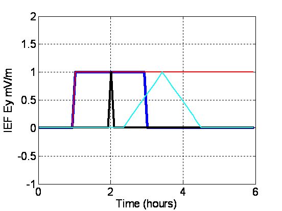

Transfer Function response to the synthetic inputs of IEF Ey. (left) The input signal and (right) the zonal electric field output (adapted from Manoj et al. [2008]).
References:
Manoj, C., S. Maus, and P. Alken (2013), Long-period prompt-penetration electric fields derived from CHAMP satellite magnetic measurements, J. Geophys. Res. Space Physics, 118, 5919–5930, doi:10.1002/jgra.50511.
Manoj, C., and S. Maus (2012), A real-time forecast service for the ionospheric equatorial zonal electric field, Space Weather, 10, S09002, doi:10.1029/2012SW000825.
Manoj, C., S. Maus, H. Lühr, and P. Alken (2008), Penetration characteristics of the interplanetary electric field to the daytime equatorial ionosphere, J. Geophys. Res., 113, A12310, doi:10.1029/2008JA013381.
Download the PPEFM model here.
We use the quiet time F-region equatorial vertical drift model by Scherliess and Fejer (1999) for the climatological part of the real-time calculator. The Scherliess and Fejer (1999) model describes the diurnal and seasonal variations in the ionospheric vertical drift for all longitudes and for all solar flux conditions. The model was derived from the incoherent scatter radar observations at Jicamarca and Ion Drift Meter observations by the Atmospheric Explorer E satellite. The vertical drift is converted to the equatorial ionospheric eastward electric field by multiplying it by the magnetic field strength along the dip equator determined from the CHAMP data (Luhr et al., 2004).
References:
Scherliess, L. and Fejer, B.G. (1999). Radar and satellite global equatorial F-region vertical drift model. Journal of Geophysical Research 104(A4): doi: 10.1029/1999JA900025.
Luhr, H., S. Maus, and M. Rother (2004), Noon-time equatorial electrojet: Its spatial features as determined by the CHAMP satellite. Journal of Geophysical Research 109 A01306: doi: 10.1029/2002JA009656.
- The model requires the interplanetary electric field (IEF), also known as the solar wind electric field, which is calculated using measurements of the interplanetary magnetic field and solar wind velocity. For real-time predictions, the primary data source is typically the Deep Space Climate Observatory (DSCOVR) satellite.
- To accurately model the impact on Earth, the IEF data must be propagated from the satellite's position to the nose of Earth's magnetospheric bow shock. For the real-time calculations, this propagation delay (Δ) is estimated assuming the solar wind travels at a constant speed (Vx) along the Sun-Earth line over the distance (ΔX) between the satellite and the bow shock nose, using the formula ΔVx. In addition to this dynamic propagation delay, we add a static, 17-minute delay [Manoj et al., 2008] to account for the IEF to travel from the bow shock's nose to the equatorial ionosphere.
- The model isn't limited to real-time; it can also calculate the EEF for any date from 1995 to the present. When calculating for dates older than approximately one month, the system switches to using interplanetary data sourced from the NASA/OMNI website. This NASA/OMNI dataset is a composite, derived from measurements by various spacecraft including ACE, Wind, IMP 8, and Geotail, and is carefully time-shifted to the Earth's bow shock nose using sophisticated phase front determination techniques.
- The climatological component of the model relies on solar flux data, specifically the 81-day moving average of the F10.7 cm solar flux, which is also obtained from SWPC data services.
- The climatological component converts vertical plasma drift (from the Scherliess & Fejer model) to electric field using magnetic field strengths from WMM at 600 km altitude along the dip equator: E (mV/m) = V (m/s) × B (nT) / 10⁶
The real-time model provides valuable predictions but is not intended to wholly represent the complex Equatorial Ionospheric Electric Field (EEF). Here are some key limitations:
- Significant day-to-day EEF variability, often reaching 0.2-0.3 mV/m even on quiet days, arises from atmospheric tides and waves originating in the lower atmosphere (terrestrial weather effects), which this model does not capture.
- The model excludes the disturbance dynamo effect, a delayed (hours to days) electric field driven by storm-time thermospheric wind changes resulting from high-latitude energy deposition, which significantly impacts the EEF during storm recovery phases.
- The transfer function assumes a linear magnetospheric response to the solar wind electric field; while a useful approximation for average conditions, this significantly deviates from reality during dynamic events like major storms or substorms.
- The non-linear processes, such as ring current dynamics, shielding/overshielding effects, and variable magnetosphere-ionosphere coupling efficiency, are not explicitly modeled, limiting accuracy during disturbed periods.
- The real-time propagation delay estimate from L1 depends primarily on solar wind velocity, without fully accounting for the interplanetary magnetic field orientation or the satellite's offset from the Sun-Earth line - factors that can introduce timing errors of ±15 minutes or more. For data older than one month, we use NASA/OMNI data, which apply a more sophisticated time-shifting method that may reduce these timing uncertainties.
- The model uses geomagnetic main field data from 2000-2010 (IGRF-2000, WMM2010, CHAMP 2004 dip equator). This may introduce an unquantified systematic error in climatological electric field values due to accumulated secular variation.
- Finally, the model's accuracy is inherently dependent on the quality and continuity of the real-time solar wind data feed, which can be subject to errors, gaps, or instrument limitations.
- JULIA radar data: The Jicamarca Radio Observatory is a facility of the Instituto Geofísico del Perú operated with support from the NSF Cooperative Agreement ATM-0432565 through Cornell University.
- NASA's OMNIWeb group for the Solar Wind data
- NOAA's Space Weather Prediction Center for the f107 and the real-time ACE and DSCOVR data sets
- Ludger Scherliess and Bela Fejer for the Climatological model
- This research was supported in part by the NOAA cooperative agreement NA22OAR4320151
User Guide: Equatorial Electric Field Model
This guide provides instructions for utilizing the Equatorial Electric Field (EEF) prediction model via the web interface and programmatic access.
I. Input Parameters (Web Interface)
Please ensure your inputs adhere to the following constraints:
- Date Range: Calculations are supported for dates from 1995-01-01 onwards. Enter dates in YYYY-MM-DD format.
- Longitude: Specify the desired longitude within the range of -180 to 180 degrees.
- Duration: Select a calculation duration between 0.125 and 5 days ( 3 hours to 5 days).
II. Data Source Selection (Advanced Options)
The model allows selection of the input solar wind data source:
- Auto (Default): This mode uses the operational NOAA SWPC Real-Time Solar Wind (RTSW) data feed for recent times (approximately the last month). This feed primarily uses DSCOVR data but automatically switches to ACE during DSCOVR outages or data quality issues.
- ACE RTSW: Forces the model to use exclusively ACE RTSW data for the entire calculation period (available from 1995 onwards).
- DSCOVR RTSW: Forces the model to use exclusively DSCOVR RTSW data (available from 2016, onwards).
Note: Using the "ACE RTSW" or "DSCOVR RTSW" options may help fill data gaps present in the standard "Auto" mode, but might include data potentially flagged as unreliable by SWPC.
III. Data Export
Model output displayed in the chart can be downloaded in CSV (Comma Separated Values) format using the "Chart Options" menu associated with the plot. Output Temporal Resolution: 5-minute intervals.
IV. Programmatic Access (API)
The model results can be accessed programmatically via HTTPS GET requests, facilitating integration into automated workflows or custom analyses.
- Base URL:
https://electric-field-dot-gbp-oit-rc-hdgmrt-app-s8g.appspot.com/ppefmL - Default Request: Sending a request to the base URL without parameters returns the real-time Prompt Penetration (PP) electric field component for all longitudes, covering the time from the request up to the maximum prediction horizon. Associated processing parameters, such as the calculated solar wind propagation delay, are also included. The output is provided in a structured format suitable for machine parsing.
- Custom Requests: Specific time periods and components can be requested using optional query parameters appended to the base URL.
- Example: To retrieve data for 3 days starting from 2003-10-20 at 20:00 UTC:
https://electric-field-dot-gbp-oit-rc-hdgmrt-app-s8g.appspot.com/ppefmL?year=2003&month=10&day=20&utc=20&nDays=3
- Example: To retrieve data for 3 days starting from 2003-10-20 at 20:00 UTC:
V. API Query Parameters
The following optional parameters can be used to customize the data request
year=<YYYY>: Specifies the year (integer, 1995-present). Default: Current year.month=<MM>: Specifies the month (1-12). Default: Current month.day=<DD>: Specifies the day of the month. Default: Current day.utc=<HH>: Specifies the start hour in UTC (0-23). Default: Current UTC hour.nDays=<days>: Specifies the duration of the data required, in decimal days (range: 0.125 to 5.0).- If
nDaysand start time (year,month,day,utc) are unspecified, data from the current time to the maximum prediction horizon is returned. - If a start time is specified but
nDaysis not, it defaults to 0.125 days (3 hours). - If the requested period (user-specified date +
nDays) extends beyond the available prediction time, data is returned only up to the end of the prediction horizon.
- If
deltalong=<degrees>: Specifies the longitude interval in decimal degrees (range: 1 to 359). Default: 18 degrees.startlong=<degrees>: Specifies the starting longitude for the data output. Default: 0 degrees.comp=<component>: Specifies the model components to return.pp: Prompt Penetration component only (Default).cl: Climatological component only.all: All components (Prompt Penetration and Climatology).
sat=<data_source>: Specifies the input data source.auto: Automatic selection (default)
Uses DSCOVR/ACE real-time for recent data
Automatically switches to OMNI for data >1 month old, 1995+ace: Force ACE RTSW satellite data (2014+).dscovr: Force DSCOVR RTSW satellite data (2016+).
VI. API Output Format
The ppefmL endpoint returns structured HTML text format containing:
- Header section: Processing metadata including data source, propagation delay, solar wind velocity, and F10.7 index
Magnetic Local Time (MLT) row: Reference MLT values for each longitude (calculated using AACGM coordinates)
Geographic longitude row: Longitude values in degrees - Time series data: Electric field values (mV/m) at 5-minute intervals, organized in rows with UT date/time stamps and columns for each longitude
- The structured text output can be parsed programmatically to extract electric field values, timestamps, and associated metadata.
VII. About This Service
- Platform: The web application and models are hosted on the University of Colorado's Google Cloud infrastructure.
- Started: December 2011, Last Updated: October 2024.
- Contact: For comments, suggestions, or assistance, please contact Manoj Nair at manoj.nair@colorado.edu